Archivo:Scattering theory illust.png
Ir a la navegación
Ir a la búsqueda
Tamaño de esta previsualización: 144 × 596 píxeles. Otras resoluciones: 58 × 240 píxeles | 480 × 1988 píxeles.
Archivo original (480 × 1988 píxeles; tamaño de archivo: 49 kB; tipo MIME: image/png)
Resumen
| Descripción |
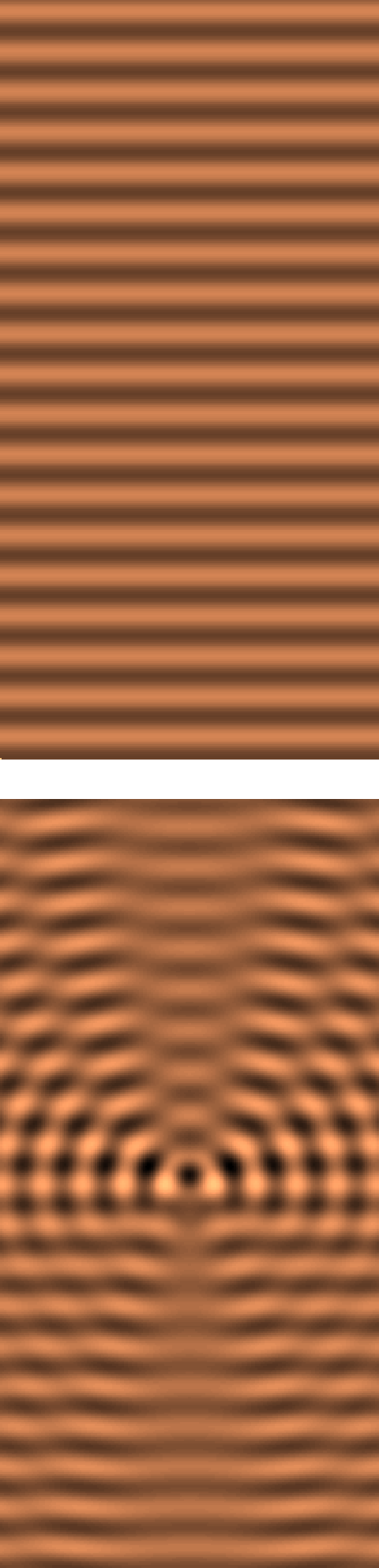
English: Illustration of Scattering theory. |
| Fecha | |
| Fuente | Trabajo propio |
| Autor | Oleg Alexandrov |
| PNG desarrollo |
Licencia
| Este trabajo ha sido liberado al dominio público por su autor, Oleg Alexandrov. Esto aplica para todo el mundo. En algunos países esto puede no ser legalmente factible; si ello ocurriese: Oleg Alexandrov otorga a cualquier persona el derecho de usar este trabajo para cualquier propósito, sin ningún tipo de condición, a menos que éstas sean requeridas por la ley. |
Source code (MATLAB)
function main(Nx, Iters)

Box_x = 3;
Scale = 0.5;
Box_y = Box_x/Scale;

%Nx = 50;
Ny = Nx/Scale;

wavenumber = 10;

XX = linspace(-Box_x, Box_x, Nx);
YY = linspace(-Box_y, Box_y, Ny);
hx = XX(2) - XX(1);
hy = YY(2) - YY(1);
[X, Y] = meshgrid(XX, YY);

Source_size  = 0.5;
Source_shift = 0;
n0=0.5;
Scatterer =  n0*sign(max(Source_size^2 - X.^2-(Y-Source_shift).^2, 0));

I = sqrt(-1);
Uinc = exp(I*wavenumber*Y);

% plot the initial planewave
figure(1); clf; hold on; axis equal; axis off; colormap copper;
Tweak=0*Uinc; Tweak(1, 1)=-2; Tweak(1, 2) = 4;
imagesc(real(Uinc)+Tweak); % a hack to have the same colormap as the images below
iter = 1;
saveas(gcf, sprintf('Scattering_frame%d_Nx%d.eps', iter, Nx), 'psc2');

%figure(3); clf; hold on; axis equal; axis off; colormap copper;
%imagesc(Scatterer);

% Approximate the Uscatter by 0
Uscatter = 0*Scatterer;

% Several iterations to improve upon the starting Born approximation
% I hope this is the right way to do things. The plotted solution looks plausible
% but I don't know if this is rigurous.

for iter=2:(1+Iters)

   % Here we use an approximate source
   Source = wavenumber^2*Scatterer.*(Uinc+Uscatter);

   % calc the solution solution to the Helmholtz equation
   Uscatter = 0*X;
   [m, n] = size(Source);
   for i=1:m
      i
      for j=1:n

	 if Source(i, j) ~= 0

	    x0 = X(i, j);
	    y0 = Y(i, j);

            % add the contribution from the current source, average over four corners of current rectangle
	    Uscatter = Uscatter ...
		+ (I/16)*(...
		   besselh(0, 1, wavenumber*sqrt((X-x0-hx/2).^2+(Y-y0-hy/2).^2) + eps)*Source(i, j) ...
		   + besselh(0, 1, wavenumber*sqrt((X-x0-hx/2).^2+(Y-y0+hy/2).^2) + eps)*Source(i, j) ...
		   + besselh(0, 1, wavenumber*sqrt((X-x0+hx/2).^2+(Y-y0-hy/2).^2) + eps)*Source(i, j) ...
		   + besselh(0, 1, wavenumber*sqrt((X-x0+hx/2).^2+(Y-y0+hy/2).^2) + eps)*Source(i, j))*hx*hy;
%Uscatter = Uscatter +(I/4)*besselh(0, 1, wavenumber*sqrt((X-x0).^2+(Y-y0).^2) + eps)*Source(i, j)*hx*hy;
	 end

      end
   end

   Utotal = Uinc + Uscatter;

   figure(1); clf; hold on; axis equal; axis off; colormap copper;
   imagesc(real(Utotal));
   saveas(gcf, sprintf('Scattering_frame%d_Nx%d.eps', iter, Nx), 'psc2');
end

|
Esta imagen debería volverse a crear como imágenes vectoriales SVG. Esto proporciona muchas ventajas, véase Commons:Media for cleanup (en inglés) para más información. Si ya hay una versión SVG de esta imagen disponible, por favor súbala a Commons. Tras subirla, reemplace esta plantilla con la plantilla
{{vector version available|nuevo nombre de imagen.svg}} en esta imagen. |
Historial del archivo
Haz clic sobre una fecha y hora para ver el archivo tal como apareció en ese momento.
| Fecha y hora | Miniatura | Dimensiones | Usuario | Comentario | |
|---|---|---|---|---|---|
| actual | 05:44 8 jul 2007 | 480 × 1988 (49 kB) | wikimediacommons>Oleg Alexandrov | Tweak |
Usos del archivo
La siguiente página usa este archivo: